[paper-review] Learning to Understand Traffic Signs

Guo, Y., Feng, W., Yin, F., Xue, T., Mei, S., & Liu, C. L. (2021, October). Learning to Understand Traffic Signs. In Proceedings of the 29th ACM International Conference on Multimedia (pp. 2076-2084).

개인적인 논문해석을 포함하고 있으며, 의역 및 오역이 남발할 수 있습니다. 올바르지 못한 내용에 대한 피드백을 환영합니다 :)

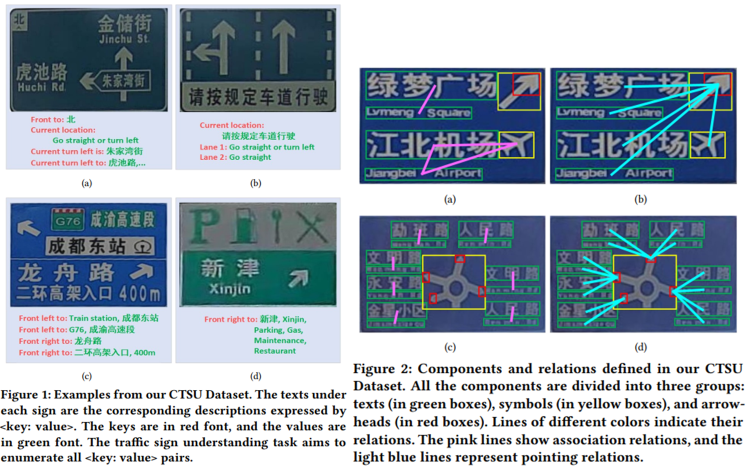
1. Introduction

최근 교통 표지판(traffic sign)에서 텍스트나 기호를 인식하는 task의 눈에 띄는 발전이 있었음
각각의 요소를 따로 인지하는 것은 교통 표지판을 이해하는 첫 단계에 불과
본 논문에서는 “traffic sign understanding”이라는 새로운 task를 소개
1. 교통 표지판에 포함된 요소들을 인식하고
2. 그 요소들 간의 관계를 파악하여
3. “semantic description”(<key: value>의 형태)을 생성하는 것
  - key: 표시 정보 (예: 현재 위치, 차선 번호, 전방 오른쪽 방향)
  - value: 특정 내용 (예: 장소 이름, 도로 이름, 설명 단어)
  - 대부분의 교통 정보가 “indicative information + content”의 형태로 구성
자율주행, positioning assistance, map correction과 같은 애플리케이션에 활용될 수 있음

img-description

[@ Traffic sign understanding]

Traffic sign understaning은 크게 세 가지 subtask로 구성
- 텍스트 및 기호의 위치와 semantic 정보를 추출하는 Component detection task
- 텍스트와 기호의 인식 결과를 어떻게 조합할 것인지, 구성요소들 간의 관계를 모델링할 수 있는 Relation reasoning task
  - Graph Convolutional Network과 같은 관계 예측 모델을 사용
- 교통 표지판의 다양한 유형을 분류하는 Sign classification task
  - 다양한 유형의 표지판에 따라같은 기호가 다른 의미를 나타낼 수 있음
  - 예) 차선 정보 표지판(그림 1(b))에서의 윗방향 화살표는 “직진”을 의미하고 안내 정보 표지판(그림 1(a))에서는 “전면”을 의미한다.
  - 교통 표지판의 유형을 예측함으로써 기호 간의 관계를 파악하는데에도 도움을 줄 수 있을 것

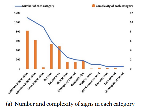
[@ CASIA-Tencent Chinese Traffic Sign Understanding Dataset (CTSU Dataset)]

복잡한 형태의 교통 표지판과 그 semantic description 레이블을 포함하는 첫 번째 데이터셋
실제 dashcam 영상에서 잘라낸 5000개의 교통 표지판 이미지를 포함
- 이미지 description, 기호, bounding box, 이미지 내의 텍스트, 기호의 카테고리
- 요소들 간의 관계에 대한 레이블도 지정

[@ Contributions]

교통 표지판 이미지 및 레이블 정보를 포함하는 데이터셋 CTSU 제안
다양한 유형의 교통 표지판을 이해하고 description을 생성하기 위한 새로운 unified 모델 제안
위 모델의 접근 방식이 traffic sign understanding에 효과적임을 실험을 통해 밝힘

2.1. Traffic Sign Recognition

이전 교통 표지판에 관한 연구는 텍스트의 detection에 관한 연구가 주를 이룸
- Peng et al. proposed a two-stage cascade detection deep learning model, which used improved EAST for text line detection, and changed the size of feature maps to suit the text size of traffic signs.
- Hou et al. introduced an Attention Anchor Mechanism (AAM), which is used to weight the bounding boxes and anchor points to detect text in scene and traffic signs.
Traffic sign에 대한 공개 datasets는 주로 원형이나 삼각형 형태의 몇몇 간단한 형태의 분류에 대해서만 존재했음
- German Traffic Sign Recognition Benchmark - citation
- DFG Traffic Sign Data Set - citation
- Chinese Traffic Sign Database (CTSD) - citation
- 위 데이터셋들은 복잡한 교통 표지판 속 요소들 사이의 관계에 대한 정보가 없음

2.2. Scene Understanding

이미지를 기반으로 semantic description을 생성하는 task를 총칭하여 image caption이라 할 수 있음
- Recurrent Neural Network (RNN) 기반
  - CNN만으로는 맥락 정보를 반영할 수 없음
  - Rowan et al. first used LSTM to predict the object categories and then sent the object features and category information into LSTM for relationship prediction.
  - Li et al. proposed a network that leveraged the feature of region, phrase, and object to generate scene graph and caption.
  - 위 연구들은 RNN이나 LSTM을 사용해 맥락 정보를 반영했음
  - 하지만, 공간적 정보(spatial information)을 반영하지 못함
- Graph Neural Network (GNN) 기반
  - 더 나은 scene graph 구조를 생성하기 위해 GNN 기반의 모델들이 제안되었음
  - Yang et al. proposed an attentional Graph Convolutional Network (aGCN) that uses contextual information to better reason about the relationship between objects
  - 이러한 방법들은 이미지 내의 맥락 정보(contextual information)를 포함할 수 있지만, 위치정보나 의미적 정보(semantic information)을 반영할 수 없음

3. CTSU Dataset

– 중략 –

3.3. Evaluation Metric

Image caption에서 이용되던 척도들은 자연어 처리에서 비롯된 척도
- 주로, 정답 값과 sequence matching의 형태이거나 유사도를 측정하는 형태
- 교통 표지판의 semantic description은 문법적인 규칙을 신경쓰지 않아도 되는 형태이므로 비효율적임

[@ Information Matching (IM)]

먼저 indicative information(<key: value>에서 key)에 대해 ground truth와 예측 값을 매칭
- 각각 예측된 predicted description에 오직 하나의 ground truth description을 매칭할 수 있음
매칭 결과에 따라 각각 specific content(<key: value>에서 value)가 일치할 때 True Positive를 부여
위 결과에 따라 각 이미지당 하나씩의 recall, precision, F1-Measure를 계산

3.4. Statistics and Analysis

CTSU Dataset contains 5,000 traffic signs
- 16,463 <key: value> descriptions
- 31,536 relationship instances
- 43,722 components, including 18,280 texts

[@ Category Statistics]

교통 표지판 클래스 별로 복잡도(Complexity)를 계산하고 이를 해석함
- 클래스 $i$에 대한 Complexity $C(c_i)$는 각 클래스 내 샘플들의 components 수($a_{c_i}$)와 각 샘플 내의 정보 엔트로피(information entropy; $H(c_i)$)의 곱으로 정의
\[\begin{matrix} C(c_i) = a_{c_i}*H(c_i) = {1\over \lvert c_i \rvert} \sum_{p\in c_i} N_p * {1\over\lvert c_i \rvert} \sum_{p\in c_i} H_p\\ H_p = -P_{pa}\log P_{pa}-P_{pp}\log P_{pp}-P_{pn}\log P_{pn}\\ \\ \text{where } \lvert c_i \rvert \text{ is the total number of images of class } i\\ N_p \text{ is the total number of components in a particular sign } p\\ P_{pa}, P_{pp}, \text{and } P_{pn} \text{ are the frequency of association relation, pointing relation, }\\ \text{and no relation in the sign } p \end{matrix}\]
CTSU 데이터셋은 샘플 수가 많은 클래스에서는 복잡도가 높고, 샘플 수가 비교적 적은 클래스에서는 복잡도가 낮음

img-description sign 클래스 당 복잡도 분석 결과

[@ Detection Imbalance]

교통 표지판 내의 구성요소들의 분포도 불균형
- ‘text’ 요소는 수가 많고 다른 요소들은 비교적 수가 적음
- 이를 잘 다룰 수 있어야 함

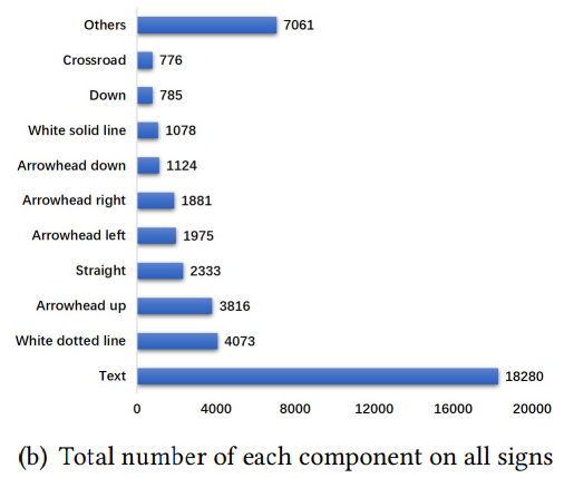
[@ Description Bias]

indicative information(<key: value>에서 key)을 담당하는 ‘text’ 요소는 20%를 미치지 못함
- ‘text’ 요소가 전체 요소의 40%를 차지함에도 불구하고
- 이 때문에 indicative information의 생성에 ‘text’의 “기여”가 과장될 것
- 과장된 ‘text’의 영향을 줄일 수 있도록 모델링해야 함

img-description indicative information을 담당하는 요소들의 분포, ‘text’ 요소는 제외함, 가장 많은 수를 차지하는 ‘Crossroad’의 수도 ‘text’ 요소에 비하면 수가 적은 편

4. Method

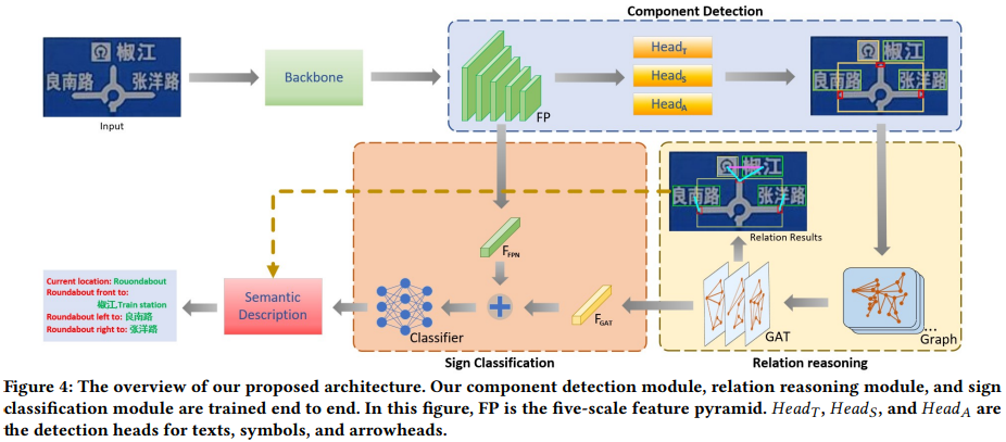img-description 논문에서 제안하는 모델의 전체 프레임워크

4.1. Component Detection

교통 표지판의 요소들을 object detector를 통해 탐지해내는 과정
single-stage anchor-freed object detection model인 FCOS를 사용
- 물체의 중앙을 기준으로 bounding box를 예측하는 FCOS 알고리즘 특성상 두 물체가 겹쳐서 존재하면 잘 탐지하지 못하는 특성이 있음
- 논문에서는 ‘texts’, ‘symbols’, ‘arrowheads’를 각각 따로따로 탐지하는 detection head를 두어 이를 해결했음
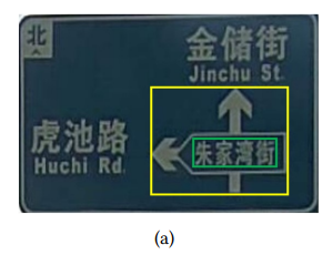\[L_{DET} = L_{FCOS_T} + L_{FCOS_S} + L_{FCOS_A}\] \[\begin{matrix} \text{where } L_{FCOS_T}, L_{FCOS_S}, \text{ and } L_{FCOS_A} \text{ are the single head losses of}\\ \text{texts, symbols, and arrowheads} \end{matrix}\]

img-description 두 요소가 겹쳐서 존재하는 경우

4.2. Relation Reasoning

그래프 구조
- 구성요소(‘texts’, ‘symbols’, ‘arrowheads’)를 그래프의 node
- 이 요소들의 관계를 그래프의 edge
- 관계를 일부 node들에 대해서만 정의할 수 없음
  - 두 요소간 물리적 거리가 가깝다고 해서 꼭 관계를 형성하지는 않음
  - 따라서, 모든 node들이 연결된 그래프 구조로 초기화

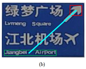img-description 관계를 형성하고 있음에도 요소간 거리가 멀리 떨어진 경우가 많음: 때문에 논문에서는 fully connected graph 구조를 사용

[@ Feature generation]

img-description

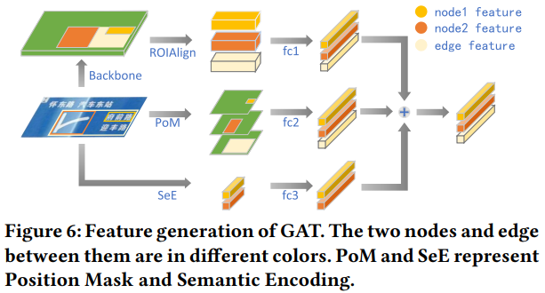
node feature 및 edge feature를 생성하는 방법
1. RoI feature: object detector가 만든 bounding box에 RoIAlign을 적용
2. Position Mask: object detector가 만든 bounding box 위치에 masking한 이미지를 fully connected layer에 연결하여 feature 생성
3. Semantic Encoding: object detector가 예측한 클래스 정보를 fully connected layer에 연결하여 feature 생성 (클래스 정보로는 edge를 표현할 수 없기 떄문에 edge에 대한 Semantic Encoding은 없다)
annotations
- node feature: $F_N = V_{ds} + V_{ps} + V_{ss}=\text{RoI feature} + \text{Position feature} + \text{Semantic feature} \in R^D$
- edge feature: $F_E = V_{du} + V_{pu}=\text{RoI feature} + \text{Position feature} \in R^D$
  - $D$는 각 feature 차원 수
- 각 feature가 업데이트 되는 것을 $\prime$을 붙임으로써 표현

[@ Graph Attention Network (GAT)]

GAT는 Graph Network에 Attention 메커니즘을 추가하여 node간 edge에 중요도를 부여하여 Graph 구조 정보를 모델링
Attention coefficient
- node $N_i$에 연관된 모든 node 및 edge에 대해 영향력이 있는 정도(중요도)를 계산
- edge $E_{ji}$는 node $N_j$에서 node $N_i$로의 관계를 의미
- $f_A: R^{2D} \to R^D$: fully connected layer
- $\parallel$: concatenation operation

\[\alpha_{ji} = {\exp(\sigma(f_A(F_{E_{ji}} \parallel F_{N_i})))\over \sum_{k\in \mathbb N_i} \exp(\sigma(f_A(F_{E_{ki}} \parallel F_{N_i})))}\]

node feature의 업데이트
- edge feature에 Attention coefficient를 element-wise 곱을 하고 node feature를 concat하여 fully connected layer에 태움
- $\otimes$: element-wise/hadamard product
- $\sigma$: activation function, 논문에서는 leaky ReLU사용
- $f_N: R^{2D} \to R^D$: fully connectec layer

\[F^\prime_{N_i} = \sigma\left(f_N\left(\left(\sum_{j\in\mathbb N_i}\alpha_{ji} \otimes F_{E_{ji}}\right) \parallel F_{N_i}\right)\right)\]

edge feature의 업데이트
- 두 노드 $N_i$와 $N_j$에 Attention coefficient를 element-wise 곱을 하고 더한 후 edge feature를 concat하여 fully connected layer에 태움
- $f_E: R^{2D} \to R^D$: fullly connected layer

\[F_{E_{ji}}^\prime = \sigma\left(f_E\left((\alpha_{ji}\otimes F_{N_j} + \alpha_{ji} \otimes F_{N_i}) \parallel F_{E_{ji}}\right)\right)\]

학습 과정에서는 ground truth bounding box를 통해 학습하여 GAT가 더 잘 수렴할 수 있게하였음

4.3. Sign Classification

교통 표지판의 관계를 파악하는데 교통 표지판의 유형을 분류하는 것이 도움이 될 수 있음
backbone feature map 중 가장 작은 feature($FP_s$)와 GAT를 거친 node feature($F_{N}$)들을 더하여 교통 표지판 유형 예측에 사용

\[\begin{matrix} F_{FPN} = f_{FPN}(Conv(Resize(FP_s))),\\ F_{GAT} = \sum_i f_{GAT}(F_{N_i})),\\ f(F_{FPN}, F_{GAT}) = f_{CLS}(F_{FPN} + F_{GAT}) \end{matrix}\]

[@ Loss Function]

section 4.1, 4.2, 4.3의 요소들의 loss를 선형 결합함

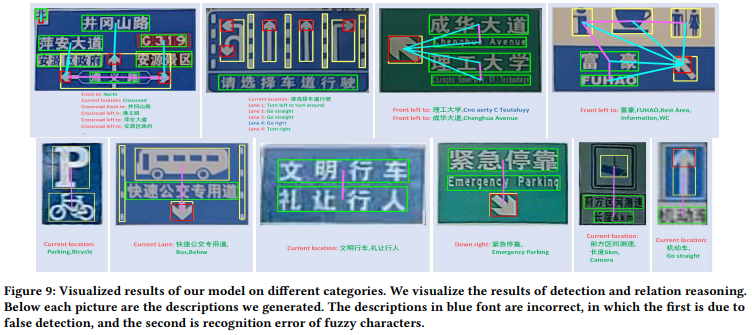
\[\begin{matrix} L=L_{DET} + \lambda_{REL}L_{REL} + \lambda_{CLS}L_{CLS}\\ \text{where } \lambda_{REL} \text{ and } \lambda_{CLS} \text{ are set to 1.0 for training.} \end{matrix}\]

4.4. Semantic Description

Inference objects
- detected box를 필터링하는 threshold = $0.2$
- relationship을 필터링하는 relationship threshold = $0.5$
- text box에 대해서는 사전학습된 OCR모델로 텍스트를 추출함
heuristic method to generate semantic descriptions
1. relation 예측 결과를 통해 relation trees를 구성
2. symbol에 따라 의미 태그 부여
  - 교통 표지판 유형에 따라 symbol에 의미를 부여
3. <key: value> structure 구성
  - 대부분 value의 위치에 명확한 요소들이 위치함 (예. 지명, 지하철역명 등등)
  - 교통 표지판 유형에 따라 key의 위치에 명확한 요소들이 위치하는 경우도 있음 (예. lane information sign에서는 차선 번호(lane 1, lane 2, …)가 key에 위치함)
  - 따라서, 해당 작업도 교통 표지판 유형에 따라 부여

5. Experiments

CTSU 데이터셋에 대해 실험 수행
학습과 검증 데이터셋에 대한 설명이 없는 것으로 봐서 아래 실험 결과는 모두 학습 데이터에 대한 실험 결과인 것으로 보인다.

5.1. Implementation Details

backbone: ImageNet에 사전학습한 ResNet-50, Deformable Convolutional Network (DCN) 테크닉 사용
GAT의 레이어 수는 5개
50 epochs
learning rate 0.01
- epoch 35, 45에 각각 0.1씩 감소
batch size 8 on 2 GPUs

5.2. Ablation Studies

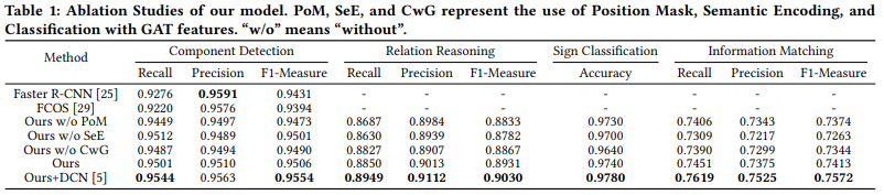
[@ Multi-head Detection]

FCOS 특성 상 겹쳐있는 물체를 포착하지 못하는 문제를 밝힘
- 약 1%정도의 성능 향상
Faster R-CNN도 겹쳐있는 물체에 대한 해결책이 될 수 있음
- 사전 정의된 anchor 세팅이 성능에 제한이 되었음
- 약 0.7% 정도의 성능 차이

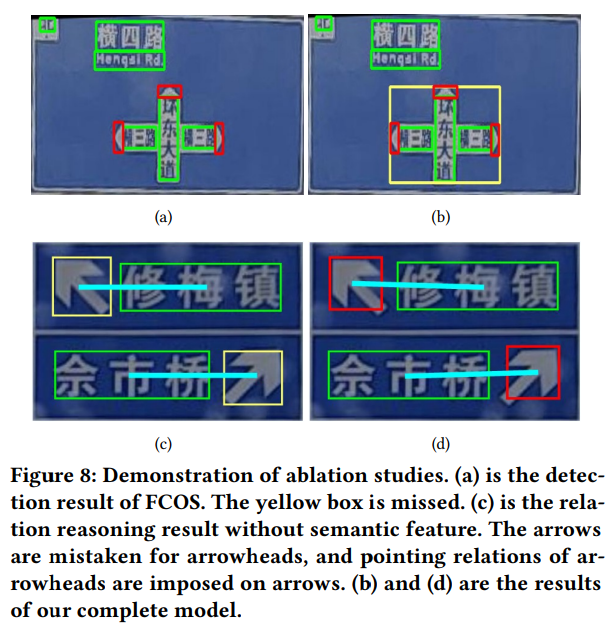img-description 기존 FCOS(a)와 논문에서 제안하는 Multi-head detection 모델(b)과의 차이

[@ Semantic Encoding]

img-description semantic feature를 제외했을 때, arrowhead가 아닌 symbol에 relation이 할당됨(c)

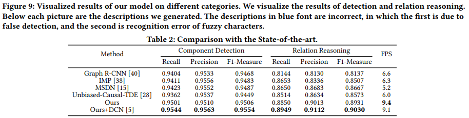
5.3. Comparison with the state-of-the-art

6. Conclusion

intelligent transportation을 위한 traffic sign understanding이라는 task를 새롭게 제안
bounding boxes, relations, semantic description 레이블을 할당한 CTSU Dataset 제안
Component detection, relation reasoning, sign classification, semantic description generation의 multi-task 학습 프레임워크를 제안